In this post, I will explain how it is possible to efficiently calculate different measures of text compressibility -- the zeroth and $k$-th order empirical entropy -- using sdsl. For both cases we use a compressed suffix tree (CST) to do the calculation. So step one is to build a compressed suffix tree of a text file. This can be easily done with the following code snippet: You can copy this program into the examples directory and execute make to get an executable, which will construct a CST for the file given by the first argument to the program. Lets take for example the file faust.txt which is located in the libraries test suite. A run of the program produces a CST names faust.txt.cst3. The CST has size 460 kB for the original 222 kB.

1 Calculating the zeroth order entropy

The zeroth order empirical entropy $H_0$ of a text $\TEXT$ of length $n$ over an alphabet $\Sigma=\{c_0,\ldots,c_{\sigma-1}\}$ of size $\sigma $ is a lower bound for a compressor which encodes each symbol independently of any of its preceding or following symbols.

\[ H_0(\TEXT) = \sum\limits_{i=0}^{\sigma-1} \frac{n_i}{n} \log{\frac{n}{n_i}} \]

where $n_i$ is the number of occurrences of character $c_i$ in $\TEXT$. It is very easy to see that $n_i$ corresponds to the size of subtree (e.g. number of leaves in the subtree) rooted at the $i$-th child of the root of the CST. The length of the text $n$ corresponds to the size of the whole tree. Therefore, the following method calculates $H_0(\TEXT)$ if v is the root node of our CST:

The code is straightforward: If the root node is a leaf, then the tree and the text are empty and $H_0$ should be 0. Otherwise we recover $n$ by determine the size of the subtree of v and calculate the first child. We then add for each child its weighted contribution to $H_0$. Note: cst.sibiling(w) returns the root node cst.root() if there is no next sibling.

2 Calculating the k-th order entropy

More advanced compressors make use of the context before a symbol and choose different codes dependent on the preceding context. Say, the length of the context is of fixed length $k$, then the $k$-th order empirical entropy $H_k(\TEXT)$ is a lower bound for compressors which encode each symbol with a codeword that depends on the preceding $k$ symbols. Here is the formal definition: \[ H_k(\TEXT) = \frac{1}{n} \sum_{\omega\in \Sigma^k} |T_\omega|H_0(T_\omega) \] where $T_\omega$ is the concatenation of all characters in $\TEXT$ which follow the occurrences of the substring $\omega$ in $\TEXT$. Note that a brute-force calculation of $H_k$ is expensive, since there are many substrings $\omega$ which do not contribute to the result, since they do not occur in $\TEXT$ and therefore $T_\omega$ is empty. Fortunately with a CST we can exactly inspect those substrings which occur in the text and can also easily calculate $|T_\omega|$ and $H_0(T_\omega)$. A substring of length $k$ is represented as a sequence of edges of length $k$ in the CST. If the substring is always followed by the same symbol $c$ then there exists no corresponding node for the substring in the CST. But in this case $H_0(T_\omega)=0$, since $T_\omega$ consists only of $c$s. On the oder hand if different occurrences of $\omega$ are followed by different characters then there exists a CST node $v$ with depth $k$. In this case $|T_\omega|$ corresponds to the size of the subtree of $v$ and $H_0(T_\omega)$ can be calculated by the algorithm from Section 1. Here is the complete code:

Example

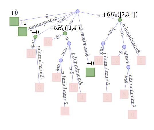
Lets look at an example. Say our string is $\TEXT$=umulmundumulmu$ and we and to calculate $H_1(\TEXT)$. Then the occurrences of substrings d, l, and n are always followed by the same character and so they do not contribute to the result. Have a look at the figure below to also note that all these substrings are not represented by a node in the CST. $ is represented by a node but does also not contribute since it is a leaf node and therefore $T_{\$}$ empty. We can also determine from the figure that the substring m is followed by one $ and four u and therefore adds $5H_0(T_m)$ to the result. Note that the actual order of characters in $T_m$ does not change the result and it is enough to know the distribution of symbols. In our case $[1,4]$. Finally, we do the same procedure also for substring u.

k-th order entropy calculation with a suffix tree

Experiment

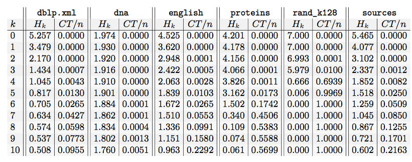
Lets take the 200 MiB test cases of the Pizza&Chili corpus build the CST with the program above and calculate $H_0,\ldots,H_{10} $ with this program:

Voilá, here is the result:

In one of the next posts, I will show that we can reach about $H_4$ in practice. If we choose larger values for $k$ then the number of contexts $CT$ is so high, that the information which is needed to store context information dominates the space.

References

Manzini's SODA article and
the full-text index overview article of Navarro and Mäkinen.
The figure and algorithms were also used as an example in my thesis.

blog comments powered by Disqus

Published

26 August 2012

Calculating the k-th order empirical entropy in linear time